The discretionary ceiling exists. Every ladder to it broke
Adding discretionary filters to my current EA, wgap, has proven to be a dead end.
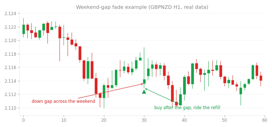
Weekend-gap fade example (GBPNZD H1, real data): trading the refill of a down gap across the weekend.
Adding discretionary filters to my current EA, wgap, has proven to be a dead end. While I identified a theoretical “oracle ceiling” where perfect manual intervention could boost monthly returns from +0.76% to as much as +1.36%, my attempts to automate these conditions failed to produce stable results.
The Discretionary Ceiling
I tested a series of discretionary brackets against the wgap system, which currently trades 10 instruments with a 68.8% win rate and a PF (profit factor: gross profit divided by gross loss) of 2.30. The “oracle ceiling” is the theoretical maximum return if a human could perfectly choose when to trade.
| Intervention Level | Monthly Return |
|---|---|
| Baseline (No intervention) | +0.763% |
| Oracle q=1/3 | +1.077% |
| Oracle q=1/2 | +1.280% |
| Oracle q=2/3 | +1.358% |
| This confirms a theoretical room for improvement of roughly 78%. However, realizing this potential through rule-based filters is a different story. |
Battery Testing and Curve Fitting
I ran 12 potential discretionary conditions through a battery test, using 400 random control samples to see if any provided a statistically significant edge. Only one condition, er_high (based on Kaufman’s Efficiency Ratio, which measures how “smoothly” price moves), survived the False Discovery Rate (FDR) test. When I applied er_high as a filter, the PF improved to 2.98, but the monthly return dropped to +0.373% because the system took fewer trades and couldn’t overcome the cost of the trade frequency. I then tried “slope sizing,” where I increased position size to 0.75% of capital when er_high was active and reduced it to 0.25% otherwise. At first glance, the numbers looked promising:
- Combined PF: Improved from 2.33 to 2.64.
- Monthly Return: Increased from +0.539% to +0.586%.
- Drawdown: Improved from -8.79% to -6.86%. However, once I split the data into IS (In-Sample) and OOS (Out-of-Sample) sets, the truth emerged. The gains were entirely concentrated in the IS period. In the OOS period, the return dropped to -2% and the max drawdown worsened. This is a classic case of curve fitting; the strategy was optimized for past data and failed to hold up against new market regimes.
Verdict
I am rejecting both the filters and the slope sizing. This aligns with my previous research showing that adding discretionary conditions to existing, high-performing sleeves usually results in over-optimization. The wgap system is most effective in its raw, low-complexity form.
Static K-Cap Sweep for Challenge Accounts
Separately, I conducted a sweep of static K-caps (the “flat guard” limit) for upcoming prop-firm challenge accounts, testing values between 2.5 and 3.0.
| K-Cap | Median Days to Pass | 1-Year Pass Rate | Failure Rate |
|---|---|---|---|
| 2.5 | 98 days | 93.7% | 16.1% |
| 2.8 | 89 days | 95.2% | 20.6% |
| 3.0 | 82 days | 96.2% | 22.6% |
| There is no internal “sweet spot” here. It is a straightforward trade-off between speed and risk. A higher K-cap helps you pass faster, but it increases the risk of disqualification during stressful market periods. For my next challenge account, I will set the K-cap between 2.8 and 3.0, while keeping my current account at 2.5. |
How this connects
This verification builds on earlier ones (what failed before and what I tried this time, comparisons between approaches).